The spelled-out intro to language modeling: building makemore
Karpathy builds a bigram character-level language model in PyTorch by counting statistics then gradient descent, showing the full training-sampling-loss loop that underpins GPT-scale models.
Key takeaways
10 points- 1A single '.' token replaces separate start/end tokens for cleaner indexing.
- 2Row normalization with keepdim=True is required for correct broadcasting.
- 3Negative log-likelihood is the standard differentiable loss for classification.
- 4One-hot encoding merely selects the corresponding row of the weight matrix.
- 5L2 regularization on weights is mathematically identical to count smoothing.
- 6torch.Generator with manual_seed guarantees reproducible sampling.
- 7All operations from one-hot to NLL are differentiable, enabling backprop.
- 8Vectorized indexing with ys avoids Python loops when computing batch loss.
- 9Zero-initialized weights produce a uniform distribution, the maximum-entropy model.
- 10The counting and neural formulations converge to the same loss surface.
Summary
Andrej Karpathy constructs a character-level bigram language model on 32k names, first via counting then via a one-layer neural net, to demonstrate the complete training, sampling and evaluation pipeline used by modern transformers.
Dataset and Bigrams
- Loads names.txt and treats each name as a sequence of characters; every consecutive pair becomes a training example (0:00-12:03).
- Maps characters to indices with s2i/i2s; adds a single '.' token for both start and end (12:04-24:05).
Counting Model
- Accumulates bigram counts in a 27x27 torch tensor N; converts to probabilities P via row normalization (12:04-24:05).
- Uses torch.multinomial with a seeded Generator for deterministic sampling of new names (24:07-36:10).
Broadcasting and Efficiency
- Pre-computes P once with torch.sum(..., keepdim=True) and broadcasting instead of looping (36:11-48:12).
Loss and Smoothing
- Evaluates quality with average negative log-likelihood; adds fake counts for smoothing to avoid zero probabilities (48:13-1:00:16).
Neural Network Formulation
- One-hot encodes inputs, multiplies by W to produce logits, applies softmax, and minimizes NLL via gradient descent (1:00:17-1:36:26).
- Shows W is exactly the log-counts matrix; L2 regularization mirrors smoothing (1:36:27-1:57:43).
Deep read
Executive Summary
This video introduces Makemore as a hands-on journey from a simple character-level bigram language model to a modern Transformer-based model, using a rigorous, step-by-step approach. Karpathy demonstrates two parallel pathways to the same learning objective: a counts-based bigram model learned by counting and normalizing Bigram probabilities, and a neural-network-based approach that learns a mapping from one-hot encoded characters to the next-character distribution via a single linear layer followed by a softmax. The talk emphasizes practical aspects: how to load data, construct and index character vocabularies, store bigram statistics in tensors for efficient sampling, and evaluate models using negative log-likelihood as a loss. It also covers optimization via backpropagation in PyTorch, sampling from the learned distributions, and smoothing/regularization to avoid zeros. The main narrative is that the neural-network framework generalizes cleanly beyond bigrams and sets the stage for scalable models (including Transformers) while preserving the same probabilistic core. The session blends theory (likelihood, log-likelihood, cross-entropy) with hands-on implementation details (one-hot encoding, tensor broadcasting, and careful handling of tensor shapes) to give the student a solid, rewatchable reference of the full pipeline: data → model → sampling → evaluation → optimization, all within PyTorch.
00:00:00 intro
Subtopic
- detailed notes / examples / explanations
- SPEAKER: Speaker: Andrej Karpathy introduces Makemore as a project to build out a language model from simple beginnings (bi-grams) toward modern Transformers. The focus of this video is twofold: (1) introduce torch.Tensor and its subtle usages for efficiently evaluating neural nets, and (2) outline the overarching language modeling framework: model training, sampling, and evaluating a loss such as the negative log-likelihood for classification.
- The video promises to evolve Makemore from a bigram character-level model to a GPT-like Transformer, with a brief roadmap toward word-level modeling and even images in future work.
- Notable idea: the sequence of work mirrors a curriculum from simple to complex networks, enabling the viewer to understand core primitives before leaping to attention-based models.
"The spelled-out intro to language modeling: building makemore" — Karpathy frames the project and sets expectations for a careful, step-by-step expansion from bi-grams to Transformers.
Notable quotes
"makemore is a repository that I have on my github webpage... it will learn to make more of things that sound name-like" (00:00:00).
Resources Mentioned
- makemore on github: https://github.com/karpathy/makemore
- jupyter notebook: https://github.com/karpathy/nn-zero-to-hero/blob/master/lectures/makemore/makemore_part1_bigrams.ipynb
- Python + Numpy tutorial from CS231n (usage note: PyTorch tensor similar to numpy array)
- PyTorch tutorials: https://pytorch.org/tutorials/beginner/basics/tensorqs_tutorial.html and https://pytorch.org/tutorials/beginner/nlp/pytorch_tutorial.html
Key Analogies / Metaphors
- Treats language modeling as building up from simple bigram probabilities to full neural nets; the analogy is a curriculum of increasing complexity where the same core ideas (probability distributions, normalization, sampling) persist.
Concepts Introduced
- Character-level language model: models sequences of characters to predict the next character.
- Bigram model: focuses on two consecutive characters; the next character depends only on the immediately prior character.
- Special tokens: start (dot) and end tokens used to frame word boundaries.
- Sampling from a model: using a probability distribution over the next character to generate sequences.
- Visualization: counts of bigrams are stored in a 28x28 matrix (later revised to 27x27), enabling intuitive sampling and inspection.
- Efficiency concept: vectorized operations and row-wise normalization to produce per-character probability distributions.
- Evaluation metric: negative log-likelihood (NLL) as a loss to measure model quality; log-likelihood is the sum of log-probabilities; NLL is its negative or the average for a dataset.
00:03:03 reading and exploring the dataset
Subtopic
- The dataset names.txt is loaded; split by lines to get a Python list of words (names).
- Observations: 32,000 names; words vary from two to fifteen characters; names contain common name-starting patterns (e.g., i, isabella) and endings (e, a).
- Framework concept: each word is a sequence of characters; the model should learn which characters are likely to follow which other characters.
- Core insight: a single word encodes multiple character-level bigrams; these carry rich statistical structure to be learned.
00:06:24 exploring the bigrams in the dataset
Subtopic
- Printing and examining two-character pairs (character1, character2) for a word to illustrate bigrams.
- Using Python’s zip to pair consecutive characters and traverse words to collect bigram statistics.
- Start token and end token: introducing start-of-word and end-of-word tokens helps to model how words begin and end.
- The bigram model captures local structure: e is likely to start many words; n often ends words; various pairs (e, n), (a, s), etc., appear with high counts.
- Transition to counting bigrams across the entire dataset via a dictionary b[bigram] += 1.
00:09:24 counting bigrams in a Python dictionary
Subtopic
- The counting approach: b at bigram increments counts for each two-character sequence (including start token -> first character and last character -> end token).
- After processing all words, print and inspect the most common bigrams (sorted by counts).
- Observations: bigram frequency reveals strong high-probability follow-ons like a followed by n, etc., consistent with name morphology.
- This stage demonstrates the simplest way to build a probabilistic model: count and normalize to produce distributions.
00:12:45 counting bigrams in a 2D torch tensor ("training the model")
Subtopic
- Shift from a Python dict to a 2D PyTorch tensor to store counts in a 27x27 (later 28x28 then 27x27) matrix, where rows correspond to the first character and columns to the second.
- Build a mapping from characters to indices (s2i) and the reverse (i2s). The alphabet includes 26 lowercase letters plus a dot (start or end) and a placeholder for the end token.
- The 2D tensor n (counts) is created with zeros of dtype int (torch int32 originally) and is incremented with the bigram counts for every word.
- Visualization: use matplotlib to display the entire 2D array and annotate with the actual bigrams to understand which pairs are common.
- Important nuance: row 0 (start dot) and column 0 (end token) are not used in most real bigrams except the start-to-first and last-to-end pairs; this leads to sparse rows/columns that can be pruned later.
- Efficiency note: plans to drop start/end redundancy and use a single special token (dot) for simplicity.
00:18:19 visualizing the bigram tensor
Subtopic
- Converts the 27x27 (or 28x28) count matrix into a human-readable visualization; i2s mapping allows labeling of each cell with the corresponding bigram.
- Observations from the visualization: some rows/columns are almost entirely zeros because certain tokens cannot begin or end a word.
- Decision: simplify to a single 27x27 matrix with a single special token (dot) at index 0; offset letters by one to make the dot pure 0 index.
- The final matrix (27x27) provides a complete, compact representation of all bigram counts after refinement.
- This matrix is all the statistical information needed to sample next characters given the current character for a bigram model.
00:20:54 deleting spurious (S) and (E) tokens in favor of a single . token
Subtopic
- Consolidation: remove separate start (S) and end (E) tokens and treat only a single dot token as the boundary marker.
- Reindex so dot is index 0; letters A..Z renamed as 1..26; this simplifies both storage and sampling.
- The resulting 27x27 matrix contains the sufficient statistics for sampling the next character given the current one.
00:24:02 sampling from the model
Subtopic
- Sampling approach: from the zeroth row (start dot), compute the probability distribution over the 27 possible next characters by normalizing the row counts to sum to 1.
- Probability vector p is created by dividing the row by its sum; then torch.multinomial is used to sample from the distribution (with replacement) to generate the next character.
- Determinism: use a PyTorch Generator seeded to get deterministic sampling across runs.
- Demonstration: draw samples (e.g., 20 samples) to produce candidate names; the results look name-like but are sometimes nonsensical, illustrating the limitations of a purely bigram model.
- Observation: if you sample from a uniform distribution, results are obviously garbage; with a trained bigram distribution, you get something more plausible but still imperfect because you lack longer-range dependencies.
- Important performance note: precompute the per-row probabilities (P) to avoid recomputing normalization in every step; this demonstrates the concept of vectorized sampling and the utility of broadcasting.
00:36:17 efficiency! vectorized normalization of the rows, tensor broadcasting
Subtopic
- To accelerate sampling and reduce redundant computations, normalize each row once to create a P matrix (27x27) where each row sums to 1.
- Tom strides through dimensions via PyTorch broadcasting: use row-wise normalization by dividing the 27x27 matrix by a column vector of row sums (27x1) so every row sums to 1.
- Broadcasting rules explained: the division is element-wise; PyTorch broadcasts the column vector across the 27 columns to produce a 27x27 normalization factor per row.
- Subtle pitfall discussed: keeping or dropping the extra dimension (keepdim) in sums changes the shape and can lead to incorrect row-wise vs column-wise normalization. A small bug emerges if the dimension handling is not careful.
- The lesson: understand PyTorch's broadcasting semantics deeply; subtle dimension mistakes can lead to incorrect normalization, effectively flipping the intended normalization axis.
00:50:14 loss function (the negative log likelihood of the data under our model)
Subtopic
- Introduce likelihood: the product of all probabilities assigned to the actual next character across the training set.
- Log-likelihood: to avoid underflow and make optimization easier, take the log of the probabilities; the log-likelihood is the sum of these log-probabilities.
- Negative log-likelihood (NLL) is defined as the negative of log-likelihood. Since we want to minimize loss, NLL is a natural choice: lower is better.
- Average NLL: sometimes we normalize by the number of examples to obtain an average loss for comparability.
- Observations: a plot of probabilities in the training set shows that some bigrams have high probability (e.g., 40% or higher) while many are small; a well-trained model assigns higher probabilities to observed bigrams and lower to unseen ones, but smoothing may be needed to avoid zero probabilities.
01:00:50 model smoothing with fake counts
Subtopic
- Problem: zero probabilities for unseen bigrams yield infinite loss; smoothing alleviates this by injecting small pseudo-counts to every bigram.
- Technique: add one to every count (Laplace smoothing) or a tunable small constant; re-normalize to obtain a valid probability distribution.
- Effect: smoothing prevents zero probabilities, keeps all bigrams assignable, and affects the sampling/generation and loss level.
- Trade-off: more smoothing makes the distribution more uniform and reduces overfitting to the observed dataset; less smoothing yields sharper, more data-driven probabilities.
01:02:57 PART 2: the neural network approach: intro
Subtopic
- Transition from explicit bigram counts to a neural network approach. The idea is to still model next-character probabilities, but use a weight matrix W and a small network to predict probabilities from inputs.
- The neural net approach aims to generalize beyond the fixed vocabulary of 27 tokens and scales better to longer contexts and larger character sets.
- The learning objective remains the negative log-likelihood of the data, now computed from the neural net's output probabilities (via softmax), and optimized by gradient-based methods.
01:05:26 creating the bigram dataset for the neural net
Subtopic
- Construct a dataset for the neural net consisting of inputs X (the first character of the bigram) and targets Y (the second character).
- Two-list representation: inputs (X) and targets (Y) are stored; later they are converted into one-hot encodings for network input.
- First word used to illustrate: EMMA; bigrams: . -> E, E -> M, M -> M, M -> A, A -> .
- Important practical note: PyTorch has two tensor constructors (torch.tensor uppercase vs torch.Tensor) with subtle differences in dtype and autograd history; prefer lowercase torch.tensor for leaves with requires_grad.
01:10:01 feeding integers into neural nets? one-hot encodings
Subtopic
- Explain one-hot encoding: convert integer class labels into one-hot vectors (27-dimensional for 27 tokens).
- Show how to use PyTorch functional one_hot to transform index tensors into one-hot form; ensure proper dtype (float32) for neural nets.
- One-hot vectors enable neural nets to operate with standard matrix multiplications: the neural net multiplies weight matrix W (27x27) by the 27-dim input, yielding a 27-dim output per example.
- The practical detail: dtype issues can arise (one_hot can produce int64 by default); cast to float32 for compatibility with neural net computations.
01:13:53 the "neural net": one linear layer of neurons implemented with matrix multiplication
Subtopic
- The neural net architecture used is a single linear layer with 27 inputs and 27 outputs (i.e., a 27x27 weight matrix W). No bias term is included initially.
- Forward pass is a matrix multiplication: outputs = X @ W, where X is a batch of one-hot-encoded inputs (e.g., 5 examples by 27 features).
- Resulting shape: 5 by 27, representing the activations (logits) of 27 output neurons for each of the 5 examples.
- Interpretation: each output neuron corresponds to a predicted count/logit for the next character; after nonlinearity, we convert logits into probabilities via softmax.
01:18:46 transforming neural net outputs into probabilities: the softmax
Subtopic
- Softmax layer: converts logits into a probability distribution over the next character for each input in the batch.
- Formula: softmax(z_i) = exp(z_i) / sum_j exp(z_j) for each input example i.
- The resulting 5x27 matrix contains probabilities that sum to 1 across the 27 tokens for each example.
- Loss function used with softmax: negative log-likelihood (cross-entropy) is computed by comparing predicted probabilities to the true next-character indices.
01:26:17 summary, preview to next steps, reference to micrograd
Subtopic
- Summary of the two modeling approaches so far: (a) a traditional bigram model learned via counts and normalization; (b) a neural-net-based approach with a single linear layer that outputs logits for the next character, followed by softmax and cross-entropy loss.
- Preview: vectorized loss, backpropagation, and updating weights via gradient descent (backpropagation) in PyTorch; then, an integrated run that ties sampling and loss together.
- Reference to micrograd shows continuity of the educational arc: introducing autograd-style computation with a small, understandable graph.
01:35:49 vectorized loss
Subtopic
- Compute the cross-entropy loss in a vectorized fashion: for a batch of five examples, gather the predicted probabilities for the true next-character indices and compute the mean negative log-likelihood across the batch.
- Use PyTorch indexing to select the predicted probabilities corresponding to the labels Y for each example, then take log, then average (or sum) to get the loss.
- The result matches the earlier scalar calculation of loss on the complete dataset; the vectorized approach is efficient and scalable.
01:38:36 backward and update, in PyTorch
Subtopic
- Backpropagation: call backward() on the loss to compute gradients with respect to all parameters (the W weights).
- Optimization step: update W using gradient descent (W = W - lr * dW).
- Demonstrate that gradients (W.grad) exist for each element, reflecting the influence of each weight on the loss.
- Re-emphasize the importance of zeroing gradients before the next pass (optimizer.zero_grad()) and the autograd mechanism that tracks the computation graph to compute gradients automatically.
01:42:55 putting everything together
Subtopic
- Integrate the forward pass (1 linear layer producing logits, softmax to probabilities), the loss calculation (negative log-likelihood), the backward pass, and the parameter update into a training loop.
- Mention that the training can be done on the entire training set of bigrams; the code scales to 228k bigrams, not just the five examples used for illustration.
- Emphasize that the objective remains consistent: minimize the negative log-likelihood to make the model assign high probability to the true next characters.
01:47:49 note 1: one-hot encoding really just selects a row of the next Linear layer's weight matrix
Subtopic
- Insight: using a one-hot input vector is equivalent to indexing into a row of the weight matrix W; hence, the neural net effectively picks a row of W corresponding to the current input token and uses that row to compute the next-token logits.
- This demonstrates that a single linear layer with one-hot inputs is essentially the same as a table lookup model with a weight matrix.
01:50:18 note 2: model smoothing as regularization loss
Subtopic
- Revisit smoothing as a form of regularization: adding a penalty to weights or counts to avoid overfitting and zero-probability issues.
- The perspective: regularization terms encourage the weights toward simpler configurations (e.g., toward zero) or toward smoother distributions.
01:54:31 sampling from the neural net
Subtopic
- Sampling from the neural net with the same mechanism as the bigram approach: encode the current token as one-hot, feed through the network to obtain logits, exponentiate to counts, normalize to probabilities, and sample the next token.
- Demonstrate that the sampling process produces sensible strings consistent with learned probabilities, albeit still imperfect, similar to the bigram sampling results.
01:56:16 conclusion
Subtopic
- Reiterate that the video demonstrates two converging paths to the same model: a bigram counts-based approach and a neural-net-based approach, both ultimately modeling the same conditional probability p(next | current).
- The neural net approach is more scalable and flexible; future videos will extend the model toward multi-character contexts, deeper networks, and eventually Transformer architectures.
- The plan is to keep the same sampling and loss framework and to grow the network capacity while preserving differentiability and the ability to compute gradients for optimization.
02:00:00 closing notes
Subtopic
- Encouragement to experiment with practice exercises (E01–E06) and to explore the community resources listed in the description (GitHub repos, notebooks, and tutorials).
- The overarching journey: from a simple bigram model to a Transformer-based language model that can generate longer passages and more coherent text, with potential extensions toward word-level modeling and multi-modal tasks like image-captioning.
Resources Mentioned (Additional)
- makemore on GitHub: https://github.com/karpathy/makemore
- makemore_part1_bigrams.ipynb: https://github.com/karpathy/nn-zero-to-hero/blob/master/lectures/makemore/makemore_part1_bigrams.ipynb
- CS231n Python + Numpy tutorial
- PyTorch Tensor Tutorials: https://pytorch.org/tutorials/beginner/basics/tensorqs_tutorial.html
- PyTorch NLP Tutorial: https://pytorch.org/tutorials/beginner/nlp/pytorch_tutorial.html
- PyTorch Functional one_hot: you can reference F.one_hot and its nuances
- Micrograd (referenced as an inspiration for step-by-step backprop)
Notable Diagrams / Visuals (Described in Words)
- A 27x27 matrix n (or 28x28 in the earlier version) with rows representing the first character and columns representing the second character; each cell contains the count of a bigram.
- A visualization showing that certain bigrams occur very frequently (e.g., n following a) while others are rare, and many rows/columns have zeros due to boundary tokens.
- A single layer neural net visualization where 27 input tokens get converted to 27 outputs via W, showing that each output corresponds to a logit for the next character, which is then exponentiated and normalized to produce probabilities.
Final Observations
- The teacher foreshadows a broader trajectory: from a bigram language model to a modern Transformer model like GPT, with the same core probabilistic framing and loss/gradient-based optimization at its heart.
- The core insight is that many different formulations (count-based vs neural-net-based) converge on the same probabilistic objective and produce similar learning signals, despite differing in scalability and expressivity.
Resources Mentioned (Recap)
- makemore on GitHub: https://github.com/karpathy/makemore
- makemore_part1_bigrams.ipynb: https://github.com/karpathy/nn-zero-to-hero/blob/master/lectures/makemore/makemore_part1_bigrams.ipynb
- CS231n Python + Numpy tutorial: https://cs231n.github.io/python-numpy-tutorial/
- PyTorch Basics Tutorial: https://pytorch.org/tutorials/beginner/basics/tensorqs_tutorial.html
- PyTorch NLP Tutorial: https://pytorch.org/tutorials/beginner/nlp/pytorch_tutorial.html
- Micrograd (reference model): a lightweight autograd-inspired approach
Topics
- Language Modeling
- Bigram
- Neural Networks
- PyTorch
- Sampling
- Regularization
- Softmax
- Negative Log Likelihood
- Gradient Descent
Action Items
- Load a names dataset and implement a pure bigram model: count bigrams, normalize per-row to obtain probabilities, and sample to generate names.
- Experiment with 2D counts tensor (27x27) and validate by sampling; compare with the dictionary-based approach.
- Implement smoothing by adding pseudo-counts to all bigrams and observe the impact on sampling and loss.
- Construct the neural-net pipeline: one-hot encode inputs, apply a 27x27 weight matrix, compute logits, apply softmax, and use cross-entropy loss on the next-character labels.
- Implement a vectorized loss calculation: gather predicted probabilities for true next-characters and compute the mean negative log-likelihood.
- Run backpropagation and gradient-based optimization on W; monitor loss and adjust learning rate to ensure stable convergence.
- Extend the neural net to take more context (e.g., trigram or longer histories) and prepare for a Transformer-based approach in future videos.
- Study PyTorch broadcasting rules carefully to avoid subtle mistakes in row/column normalization and ensure consistent semantics.
Mental Models
Glossary
- Bigram
- A sequence of two consecutive symbols (here, two characters) used to model the probability of the next symbol given the current one.
- Trigram
- A sequence of three symbols; used in higher-order language models where the next word/character depends on the two previous ones.
- One-hot encoding
- Represent a discrete class with a vector of zeros except for a single one in the index corresponding to the class.
- Softmax
- A function that converts a vector of real-valued scores (logits) into probabilities that sum to one; used for multi-class classification.
- Cross-entropy
- A loss function measuring the difference between predicted probability distribution and the true distribution (labels). For classification, it is the negative log-likelihood of the true class.
- Negative log-likelihood (NLL)
- The negative of the log-likelihood; a common loss for probabilistic models, especially with softmax outputs.
- Broadcasting
- A method by which tensors of different shapes are automatically expanded to a common shape for element-wise operations.
- logits
- The raw, unnormalized scores produced by a neural network before applying softmax to obtain probabilities.
- Laplacian / smoothing
- Techniques to prevent zero probabilities by adding small constants to all counts or priors.
- Backpropagation
- The algorithm to compute gradients of the loss with respect to model parameters by traversing the computation graph backward.
- Transformer
- A neural network architecture based on attention mechanisms that scales to long-range dependencies; mentioned as the future goal of Makemore.
- Neural network
- A computational model comprised of layers of neurons with learnable weights, capable of representing complex mappings from inputs to outputs.
- Tensor
- A multi-dimensional array used in PyTorch for data storage and computations; can be manipulated with vectorized operations.
Notable Quotes
“> makemore is a repository that I have on my github webpage... it will learn to make more of things like this”
“> here are some example generations from the neural network... dontel irot zhendi”
“> a very simple and weak language model but it's a great place to start”
“> this bigram language model... is basically a two-character diagram”
“> we start with dot the start token and we grab the first row”
“> sampling from the model... we will sample from the distribution”
“> the more we sample the more these numbers should roughly have the distribution here”
“> loss is the negative log-likelihood”
“> model smoothing as regularization loss”
“> the neural net approach... is to take the previous character and feed it through a linear layer”
“> the forward pass is differentiable and backpropagable”
“> these two approaches converge on the same objective”
“> and this w is the log counts of what we've estimated before”
Topics
More from Neural Networks: Zero to Hero
See all