Building makemore Part 2: MLP
Implements a character-level MLP language model from Bengio et al. 2003, covering embeddings, cross-entropy, learning-rate search, and train/val/test splits to surpass bigram baselines.
Key takeaways
10 points- 1Replace one-hot × matrix multiply with direct embedding-table lookup.
- 2Use F.cross_entropy for fused, numerically stable loss.
- 3Run a learning-rate sweep on a log scale to locate the stable valley.
- 4Always hold out validation and test sets before tuning.
- 5Monitor train/dev gap to diagnose under- or over-fitting.
- 6Increase hidden-layer width when both losses plateau.
- 7Visualize embeddings to verify the model has learned meaningful similarities.
- 8Initialize so that initial loss ≈ -log(1/vocab_size).
- 9Mini-batches give noisy but sufficient gradients and far more steps per wall-clock second.
- 10Reproduce results in Colab when local environment setup is costly.
Summary
Karpathy implements the Bengio 2003 MLP language model for character-level next-token prediction.
Bengio MLP Architecture
- Context of 3 characters is embedded via a shared 27×30 lookup table C and concatenated (0:00-12:02).
- Hidden layer applies tanh; output logits feed softmax (24:08-36:09).
Efficient PyTorch Internals
viewreinterprets storage without copies;F.cross_entropyfuses kernels and stabilizes large logits by subtracting the max (24:08-36:09).
Training Loop & Mini-Batches
- Zero gradients, backward, step with learning rate; 32-example batches give noisy but useful gradients (36:10-48:11).
Learning-Rate Finder
- Sweep 10^-3 to 10^0; valley around 0.1 yields fastest stable descent (48:12-1:00:17).
Data Splits & Overfitting
- 80/10/10 train/val/test prevents memorization; validation tunes hyperparameters (48:12-1:00:17).
Scaling & Visualization
- Larger hidden layer (300 neurons) and 2-D embedding plots reveal vowel clusters; further gains require bigger embeddings (1:00:18-1:12:21).
Deep read
Executive Summary
Andrej Karpathy’s Building Makemore Part 2: MLP guides the evolution from a simple bigram approach to a neural, character-level language model built around embeddings and a multilayer perceptron. The talk walks through the Bengio et al. 2003 framework, adapting it to characters, and emphasizes that each token (character) is mapped to a learnable dense vector (embedding) which, when concatenated and processed through a hidden layer, yields a probabilistic distribution over the next character via a softmax. Practical engineering details are foregrounded: dataset construction with a fixed context length (block size), embedding matrices, tensor reshaping, and the distinction between concatenation vs view-based reshaping for efficient matrix multiplication. The lecture then dives into the loss (negative log likelihood via cross-entropy), the advantages of PyTorch’s F.cross_entropy (fused kernels, numerical stability, simpler backprop), and a working training loop with minibatching, learning-rate discovery, and LR decay. The workflow extends to training on the full dataset, evaluating on dev and test splits, exploring larger hidden layers and embedding sizes, and finally sampling from the trained model to generate text. A Colab notebook is advertised to lower barriers for experimentation. The video ends by inviting readers to beat the presented 2.17–2.3 dev losses through iterative hyperparameter tuning and scale-up experiments, while noting the perils of overfitting and the importance of three-way data splits.
Key themes include: the transition from count-based representations to learned embeddings, the practicalities of embedding-based neural networks for sequence modeling, the critical role of data splits and hyperparameter tuning, and the practicalities of training and sampling in PyTorch. The content also serves as a concrete bridge to Bengio’s 2003 ideas, illustrating how to implement them in modern tooling and how to reason about model capacity, data scale, and optimization strategies in pursuit of better, more generalizable character-level language models.
00:00:00 Introduction
Speaker: Andrej Karpathy
- This video continues Makemore with a shift from a bigram model to a multilayer perceptron (MLP) language model at the character level. The goal is to predict the next character given a context, but with a neural network rather than a counts-based table.
- Key themes include: how to train a model, learning rate tuning, hyperparameters, evaluation, train/dev/test splits, and core ML concepts like overfitting vs. underfitting. The presenter emphasizes practical engineering details (data preprocessing, embedding lookup, tensor storage, optimizers) alongside theoretical ideas.
Notable quote: "the problem with this model of course is that if we are to take more context into account when predicting the next character in a sequence things quickly blow up" (00:00:00–00:01:48 region)
- The video frames the shift from a simple bigram (one previous character) to using a network with context windows and embeddings – a foundational step toward scalable neural language models.
00:01:48 Bengio et al. 2003 (MLP language model) paper walkthrough
- The presenter introduces Bengio et al. 2003 as a foundational paper in neural language modeling. The model in the paper is word-level, but the same architectural intuition applies to character-level modeling.
- Core idea: embed discrete tokens (words in the paper; characters here) into continuous vectors, then feed those embeddings through a multi-layer network to predict the next token.
- The embedding concept is central: each token (word) is mapped to a dense vector in a lower-dimensional space (for example, 30 dimensions for 17,000 words). The embeddings start random and are tuned via backpropagation.
Notable quote: "basically they propose to take every one of these words and they're going to associate to each word a say thirty dimensional feature vector" (00:01:48 region)
- Analogy used: the embedding space acts as a crowded but structured space where semantically similar words cluster together, enabling generalization to phrases not seen verbatim in training (e.g., transfer of knowledge via embeddings when encountering novel phrases).
- The network diagram: three previous words (context) become 90 inputs (3 words × 30-d embedding). These are concatenated into a single vector, fed into a hidden layer, and then into an output layer with 17,000 units (one per possible next word), followed by a softmax to produce a probability distribution over the next token.
- The training objective mirrors the classic maximum likelihood principle: maximize the log likelihood of the training data (equivalently minimize cross-entropy loss with the true next token).
- The talk emphasizes the intuition that embeddings enable generalization in out-of-distribution contexts by placing semantically related words near each other in embedding space.
Notable quote: "they are using a multi-layer neural network to predict the next word given the previous words and to train the neural network they are maximizing the log likelihood of the training data" (00:01:48 region)
00:09:03 Re-building the training dataset
- The dataset construction script is introduced, focusing on creating a context (block) of a fixed size (block size = 3 in the example) to predict the next character.
- The data creation process builds x (inputs) and y (labels) as sequences where each x is a sliding window of context tokens and y is the subsequent character.
- Padding is used (with dots) to manage the start of sequences; the block size determines how many prior characters are used to predict the next one.
- The dataset excerpt shown yields a demonstration of how emma, etc., generate multiple training examples from a given contiguous text. The result is a dataset of 32 examples for the current five words example, each input being three integers (indices) and the label a single integer (the next character).
Notable quote: "we're taking three characters to predict the fourth one and we're always padding with dots" (00:09:03 region)
00:12:19 Implementing the embedding lookup table
- The dataset now uses a character vocabulary (e.g., 27 possible characters). An embedding lookup table C of shape [vocab_size, embedding_dim] maps each character index to a dense vector.
- The embedding dimension is a design choice (the paper’s analogy uses 30; the tutorial example uses 2–30 in different experiments). The embedding table is learnable and updated via backpropagation.
- Embedding mechanics are demonstrated: indexing into the embedding matrix with a tensor of character indices yields a corresponding tensor of embeddings with shape [batch_size, block_size, embedding_dim].
- Two equivalent viewpoints are discussed: (a) indexing into C to retrieve the embeddings, or (b) encoding indices as one-hot vectors and multiplying by C. The practical approach is to index into C directly, which leverages PyTorch’s advanced indexing.
Notable quote: "embedding lookup table c this lookup table is a matrix that is 17 000 by say 30" (00:12:19 region)
- A crucial PyTorch detail: you can index C with a 2-D or 3-D tensor of indices to simultaneously embed the entire input batch, preserving efficiency.
- The talk includes a practical note on data types: one-hot encoding yields a long tensor that you can multiply by C after casting to float; however, indexing into C is more efficient and conceptually equivalent.
00:18:35 Implementing the hidden layer + internals of torch.Tensor: storage, views
- The hidden layer design: after embedding, the 3×embedding_dim vectors are concatenated into a single 1D vector per example (size block_size × embedding_dim) to feed into a fully connected hidden layer of size H (e.g., 100).
- The lecture delves into tensor shapes and the importance of shaping: [batch_size, block_size, embedding_dim] needs to be reshaped to [batch_size, block_size × embedding_dim] for the linear transformation.
- PyTorch internals: tensors are backed by a 1-D storage (the actual memory). “View” is a cheap, zero-copy operation that reinterprets the same memory with a different shape, while “concat” actually allocates new memory.
- A comparison is drawn between two concatenation strategies: (a) explicitly concatenating via torch.cat (which allocates new memory) versus (b) viewing the tensor as a flattened 2D array (e.g., 32×6) to perform a single matrix multiply without repeated allocations.
- Efficiency note: using view to reinterpret shapes is dramatically faster than concatenating; however, concatenation can be necessary if you truly need to combine tensors in a way that cannot be captured by a view.
Notable quote: "embedding a single integer like 5 is easy... indexing into row five" (00:18:35 region)
- The walkthrough shows how to build a small 32×3×2 example, then reshape to 32×6 to feed into an MLP with a hidden layer of 100 neurons, followed by a nonlinearity and an output layer.
- The discussion also covers the subtlety of broadcasting a bias term across the minibatch correctly; PyTorch broadcasting aligns on the right, so a [1×100] bias broadcasts to [32×100].
00:29:15 Implementing the output layer
- The output layer maps from the hidden layer of size H to the vocabulary size V (e.g., 27 in the character example). This is a fully connected layer with weights W2 of shape [H, V] and a bias b2 of shape [V].
- The forward pass yields logits of shape [batch_size, V], which are unnormalized log probabilities for the next character.
- The raw logits are turned into a probability distribution via a softmax (an exponential normalization) to produce probabilities across the V potential next characters for each example in the batch.
- The target next character indices (y) are then used to select the predicted probability for the correct class, enabling the cross-entropy (negative log-likelihood) loss to be computed.
Notable quote: "logits which are the outputs of this neural net are going to be 32 by 27" (00:29:15 region)
00:29:53 Implementing the negative log likelihood loss
- The initial approach computes the probability of the correct next character for each example in the batch and then computes the negative log likelihood (NLL) loss as the negative log of these probabilities. This is equivalent to cross-entropy loss for a classification task with a single correct class per example.
- The lecture then shows how PyTorch’s functional API provides a built-in, numerically stable cross-entropy function (F.cross_entropy) that combines log-softmax and negative log likelihood for stability and efficiency.
- Benefits of using F.cross_entropy include fused kernels, better numerical stability (softmax overflow prevention via log-sum-exp trick), and a simpler backward pass for optimization.
Notable quote: "there is a functional.cross_entropy function in PyTorch to calculate this much more efficiently" (00:32:49 region) [note: the exact timestamp in transcript is 00:32:49 for the cross-entropy intro; the essence is at 00:32:49 region]
00:32:17 Summary of the full network
- Recap of architecture: context window (block size) of characters embedded via C into dense vectors, concatenated into a single vector, passed through a hidden layer, then to a large output layer with V logits, followed by softmax to yield probabilities for the next character.
- The training objective is to minimize the cross-entropy (negative log likelihood) loss between the predicted distribution and the actual next character.
- Data preparation, embedding, the hidden layer, and the output layer all contribute to the learnable parameters that get updated via backpropagation.
Notable quote: "the full network" (00:32:17 region)
00:32:49 Introducing F.cross_entropy and why
- A deeper dive into the rationale for using F.cross_entropy: (1) fused kernels reduce memory allocations and speed up computation, (2) the backward pass is simpler with an analytically derived gradient, (3) numerically more stable due to the log-softmax trick that subtracts the maximum logit to prevent overflow.
- The concept of numerical stability is illustrated with a discussion on how large positive logits can overflow, while cross-entropy with log-softmax mitigates this by offsetting logits by their maximum value.
Notable quote: "this offset is a trick that makes the calculation stable... PyTorch will subtract the maximum value" (00:36:10 region)
00:37:56 Implementing the training loop, overfitting one batch
- The video demonstrates a simple training loop: compute loss on a minibatch, zero gradients, backpropagate to compute gradients, and update parameters with gradient steps.
- The initial demonstration shows how the model can quickly overfit a single tiny batch (e.g., 32 examples) due to the relatively small dataset and a reasonably large parameter count. This is an expected phenomenon: with enough capacity, a network can memorize small datasets.
- The lecture emphasizes that overfitting on a single batch is not a flaw of the model per se; it is a natural consequence of dataset size vs. model capacity and motivates the need for train/validation/test splits.
Notable quote: "it's very easy to make this neural net fit only these two 32 examples because we have 3,400 parameters and only 32 examples" (00:37:56 region)
00:41:25 Training on the full dataset, minibatches
- With a larger dataset (hundreds of thousands of examples), training on a single batch is not feasible or meaningful. A minibatch approach is introduced: randomly sample a small batch of indices to construct the minibatch, then perform forward, backward, and update steps.
- The importance of minibatching is explained: it provides a reasonable approximation to the true gradient while allowing many updates per second, enabling more efficient learning.
- The presenter emphasizes the practical workflow: begin with a small model, observe training vs. validation performance, and adjust architecture and hyperparameters to improve generalization.
Notable quote: "in practice you forward and backward on many batches... this is how you train effectively" (00:41:25 region)
00:45:40 Finding a good initial learning rate
- A pragmatic approach to learning rate selection is demonstrated: scan a range of learning rates and observe how the loss behaves across a short training run.
- The speaker tests several candidates (ranging across orders of magnitude) and plots the resulting loss, looking for a sweet spot where the loss decreases smoothly without instability or divergence.
- Conceptually, smaller learning rates result in slower but stable convergence, while too-large rates cause oscillations or divergence; an intermediate rate is often found by empirical search.
Notable quote: "this is one way to determine a reasonable set of hyperparameters... you see how the loss decreases" (00:45:40 region)
- The technique shown includes a logarithmic sweep over learning rates (10^exponent) to efficiently explore several orders of magnitude and identify a robust starting point (often around 0.1 for many small-scale models).
- After identifying a reasonable rate, a learning rate schedule (decay) is introduced to fine-tune toward convergence.
00:53:20 Splitting up the dataset into train/val/test splits and why
- The video introduces the three-way data split standard in ML:
- Training set: used to optimize model parameters (weights and biases). - Development/Validation set: used to tune hyperparameters (hidden layer size, embedding size, regularization, learning rate schedule, etc.). It guards against overfitting to the training data and helps select the final model configuration. - Test set: used to evaluate the final performance of the model after hyperparameters have been fixed, to give an unbiased estimate.
- The rationale is emphasized: with a single split (train only), you risk overfitting to the data and reporting overly optimistic results; with a proper train/val/test split, you can better assess generalization.
Notable quote: "three splits: train, dev/validation, and test" (00:53:20 region)
01:00:49 Experiment: Larger hidden layer
- An experiment increases the hidden layer size to probe capacity and its effect on performance. The number of parameters grows (more weights between the hidden layer and the embedding inputs, plus biases).
- The speaker discusses practical concerns: larger networks require more data to avoid overfitting; when data is limited, you can overfit; you may need to adjust batch size and learning rate accordingly.
- The goal is to observe if increasing capacity yields lower training and validation losses, or if it introduces diminishing returns or overfitting tendencies.
Notable quote: "experiment: larger hidden layer" (01:00:49 region)
01:05:27 Visualizing the character embeddings
- The embedding vectors for characters are visualized in 2D when embedding_dim is small (e.g., 2). This provides intuition about how the model groups characters semantically (e.g., vowels clustering together; rare letters and punctuation like ‘q’ or dot being outliers).
- The visualization reveals that the network learned structured relationships: vowels cluster, punctuation occupies distinct regions, and oddities like dot appear far away (reflecting usage patterns in the data).
- This section serves as an empirical sanity check: embeddings carry meaningful structure after training, suggesting the model is capturing useful relationships.
Notable quote: "the network has basically learned to separate out the characters and cluster them a little bit" (01:05:27 region)
01:07:16 Experiment: Larger embedding size
- The embedding size is increased (e.g., from 2 to 10 dimensions) to test whether higher-capacity token representations improve performance and help the model capture more nuanced relationships among characters.
- The hidden layer dimensionality is adjusted correspondingly to accommodate the larger input (more inputs to the hidden layer, more parameters). The initial results show that simply increasing embedding size can help mitigate bottlenecks and improve the model's ability to fit the data, though it also increases training cost.
Notable quote: "embedding size ... we’re taking as input 3×10 so 30 inputs will go into the hidden layer" (01:07:16 region)
- The talk emphasizes the interplay between embedding dimensionality and model capacity: a too-small embedding space can bottleneck performance even if the rest of the network is large; conversely, very large embeddings require careful regularization and more data.
01:11:46 Summary of our final code, conclusion
- The presenter recaps the overall pipeline and iterates on the idea that the single-step bigram model is insufficient for realistic language generation; the MLP with embeddings is a principled next step.
- It is highlighted that the network can be improved by adjusting hyperparameters (hidden size, embedding size, context window), data scales, and optimization strategies (learning rate schedules, mini-batch sizes).
- The discussion also emphasizes practical experimentation culture: run many variants, compare dev performance, and converge on a model that generalizes well rather than memorizing training data.
Notable quote: "now we invite you to beat this number and you have quite a few knobs" (01:11:46 region)
01:13:24 Sampling from the model
- The video demonstrates how to sample from the trained model to generate text. The process begins with a context of dots (an initial placeholder), then iteratively:
1) embed the current context using the embedding table C, 2) project to the hidden state, compute logits for the next character, apply softmax to obtain a probability distribution, 3) sample the next character index from this distribution (multinomial sampling), 4) append the sampled character to the context and continue.
- The generated samples appear more word-like as training progresses, demonstrating qualitative improvements in the model’s ability to produce plausible sequences.
Notable quote: "sampling from the model" (01:13:24 region)
01:14:55 Google Colab (new!!) notebook advertisement
- An advertisement for a Colab notebook that enables running the same code in a browser without local installation. The Colab notebook allows training, plotting, and sampling in an accessible environment, lowering barriers to experimentation.
12:03 Deep Dive: Dataset construction (interpolated cross-section)
- A closer look at the dataset construction code (interleaved in the talk) shows how the sliding window (context block) is built and how x (input indices) and y (target indices) are populated for training. The code includes padding and rolling context windows to illustrate how a sequence is transformed into many training examples.
Resources Mentioned
- makemore on GitHub: https://github.com/karpathy/makemore
- makemore_part2_mlp notebook: https://github.com/karpathy/nn-zero-to-hero/blob/master/lectures/makemore/makemore_part2_mlp.ipynb
- Colab notebook (new): https://colab.research.google.com/drive/1YIfmkftLrz6MPTOO9Vwqrop2Q5llHIGK?usp=sharing
- Bengio et al. 2003 MLP language model paper: https://www.jmlr.org/papers/volume3/bengio03a/bengio03a.pdf
- karpathy.ai: https://karpathy.ai
- karpathy on Twitter: https://twitter.com/karpathy
- Neural Networks: Zero to Hero Discord: https://discord.gg/3zy8kqD9Cp
- PyTorch internals: http://blog.ezyang.com/2019/05/pytorch-internals/
Exercises
- E01: Tune the hyperparameters of the training to beat my best validation loss of 2.2
- E02: Initialization sensitivity questions: (1) loss with perfectly uniform predicted probabilities at initialization; (2) tune initialization to make the starting loss closer to that baseline
- E03: Read Bengio et al. 2003 and implement any idea from the paper; test its effect
Chapters (timed list)
- 00:00:00 intro
- 00:01:48 Bengio et al. 2003 (MLP language model) paper walkthrough
- 00:09:03 (re-)building our training dataset
- 00:12:19 implementing the embedding lookup table
- 00:18:35 implementing the hidden layer + internals of torch.Tensor: storage, views
- 00:29:15 implementing the output layer
- 00:29:53 implementing the negative log likelihood loss
- 00:32:17 summary of the full network
- 00:32:49 introducing F.cross_entropy and why
- 00:37:56 implementing the training loop, overfitting one batch
- 00:41:25 training on the full dataset, minibatches
- 00:45:40 finding a good initial learning rate
- 00:53:20 splitting up the dataset into train/val/test splits and why
- 01:00:49 experiment: larger hidden layer
- 01:05:27 visualizing the character embeddings
- 01:07:16 experiment: larger embedding size
- 01:11:46 summary of our final code, conclusion
- 01:13:24 sampling from the model
- 01:14:55 google collab notebook advertisement
NOTE on visuals and diagrams
- Beta diagrams described in the talk include: a diagram of three-context words feeding into a 30-d embedding per token, concatenation of embeddings into a 90-d vector, a hidden layer, and a 17,000-unit output layer with a softmax. The embedding visualization in 2D demonstrates clustering of characters (e.g., vowels grouped together) after training, illustrating the semantic structure learned by the model.
Notable lines (verbatim quotes)
"the problem with this model of course is that you only take one character of previous context" (00:00 region) "they have a vocabulary of 17 000 possible words and they instead build a word level language model but we're going to still stick with the characters but we'll take the same modeling approach" (00:01:48 region) "embedding lookup table c this lookup table is a matrix that is 17 000 by say 30" (00:12:19 region) "logits which are the outputs of this neural net are going to be 32 by 27" (00:29:15 region) "there is a functional.cross_entropy function in PyTorch to calculate this much more efficiently" (00:32:49 region) "it's very easy to make this neural net fit only these two 32 examples because we have 3 400 parameters and only 32 examples" (00:37:56 region) "in practice you forward and backward on many batches... this is how you train effectively" (00:41:25 region) "this is one way to determine a reasonable set of hyperparameters... you see how the loss decreases" (00:45:40 region)
Glossary (selected terms defined in plain language)
- AI/ML term + simple definition: See the glossary section for a full list with clear, plain-language definitions integrated into the reading.
Final notes
- The video emphasizes practical ML engineering: from data preparation and embedding choices to learning rate scouting and proper data splits. The learner is encouraged to run experiments, observe dev-set performance, and iterate toward better-generalizing models.
- The Colab notebook offer lowers the barrier to experimenting, aligning with the open-source, hands-on ethos of the Makemore project and Karpathy's Zero to Hero series.
Quick takeaways
- Embedding-based MLPs provide a scalable way to model next-token prediction with context; embeddings generalize to unseen contexts.
- Data splits (train/val/test) are essential for assessing real performance and avoiding overfitting on training data.
- PyTorch features (e.g., embedding lookups, F.cross_entropy, and tensor view vs. concatenation) enable efficient and clean implementation.
- Hyperparameter tuning (hidden size, embedding size, block size, learning rate, batch size) dramatically impacts learning efficiency and generalization; the process often involves systematic experiments and sometimes LR-finding sweeps.
Topics
- MLP Language Model
- Character Embeddings
- PyTorch Embedding Internals
- Training, Validation, and Testing Splits
- Hyperparameter Tuning and Learning Rate Scheduling
- Sampling from Neural Language Models
- Model Evaluation and Overfitting vs. Underfitting
Action Items
- Implement train/validation/test splits for any language-modeling dataset and ensure a clean evaluation protocol.
- Experiment with embedding dimensions (e.g., 2, 10, 30, or higher) and analyze their impact on dev loss and sampling quality.
- Vary the hidden layer size (e.g., 100, 200, 300) and observe changes in training dynamics and generalization.
- Extend the block size to study longer context effects on next-character predictions.
- Perform an LR-finding sweep: test exponentially spaced learning rates (e.g., 0.001 to 1.0) and pick a stable region for training.
- Use F.cross_entropy for training and compare with a manual cross-entropy implementation to observe gains in performance and stability.
- Visualize embeddings to inspect clustering and identify potential bottlenecks in low-dimensional spaces.
- Train a larger model on a larger dataset and monitor for overfitting; consider regularization if needed.
- Implement and test a learning-rate decay schedule (e.g., multiply by 0.1 after certain iterations) and compare convergence behavior.
- Run the provided Colab notebook to replicate results and iterate quickly on hyperparameters without local setup.
Mental Models
Glossary
- MLP
- Multilayer Perceptron: a feedforward neural network with at least one hidden layer that transforms inputs through linear mappings and nonlinear activations.
- embedding
- A dense vector representation of a discrete token (e.g., character, word) learned during training that captures semantic or contextual similarity.
- logits
- The raw, unnormalized scores produced by a model before applying softmax to obtain probabilities.
- softmax
- A function that converts a vector of real numbers into a probability distribution that sums to 1, emphasizing the largest values.
- cross-entropy
- A loss function measuring how well predicted probabilities match the true distribution; for a single class in classification, it aligns with negative log likelihood.
- negative log likelihood (NLL)
- The negative log of the probability assigned to the true class; minimized during training.
- minibatch
- A small, random subset of the training data used to compute an approximate gradient for iterative optimization.
- overfitting
- When a model learns the training data too well, including noise, and fails to generalize to unseen data.
- underfitting
- When a model is too simple to capture underlying patterns, resulting in poor performance on both training and unseen data.
- train/dev/test split
- Partitioning data into three sets: training (to optimize parameters), development/validation (to tune hyperparameters), and test (to evaluate final performance).
- embedding_dim
- The dimensionality of the dense vector used to represent each token in the embedding space.
- block size
- The number of previous tokens used as context for predicting the next token.
Topics
More from Neural Networks: Zero to Hero
See all