Building makemore Part 4: Becoming a Backprop Ninja
Manually deriving every gradient through a 2-layer MLP with BatchNorm replaces PyTorch autograd and reveals exactly how gradients flow through cross-entropy, linear layers, tanh and normalization.
Key takeaways
10 points- 1Manual backprop removes the autograd black box and surfaces subtle gradient bugs.
- 2dlog_probs receives -1/N only at the correct class indices; everything else is zero.
- 3Forward broadcast implies backward summation along the identical axis.
- 4Analytic cross-entropy gradient is simply softmax_probs minus the one-hot label vector.
- 5Bias gradients are obtained by summing the upstream gradient across the batch dimension.
- 6BatchNorm backprop must accumulate contributions from mean, variance and centering paths.
- 7Bessel’s correction (n-1) is preferred for unbiased variance despite train-test mismatch.
- 8Dimensional analysis instantly reveals the correct transpose placement for matrix gradients.
- 9The complete manual backward pass for the MLP fits in roughly 20 lines of code.
- 10Verification against torch.autograd.grad yields differences on the order of 1e-9.
Summary
A hands-on derivation of the full backward pass for a two-layer MLP with BatchNorm, showing how to replace loss.backward() with explicit gradient code.
Why manual backprop matters
- PyTorch autograd is a leaky abstraction; without internals knowledge, bugs in gradient clipping, dead neurons or exploding/vanishing gradients are hard to diagnose (0:00-12:02).
- Historical papers (2006 RBMs, 2014 fragmented embeddings) implemented backward passes by hand, proving the skill remains relevant.
Loss and cross-entropy gradients
- dlog_probs is initialized to zeros then set to -1/N only at the correct indices; all other entries stay zero (12:03-24:06).
- Analytic cross-entropy yields delogits = P - 1 for the correct class and P otherwise; the sum of each row is exactly zero (1:24:26-1:36:28).
Element-wise ops, broadcasting and reuse
- Forward broadcast implies backward summation along the same dimension; reuse of any tensor requires += accumulation of its gradients (24:08-36:11).
- Operations added purely for numerical stability (logit_maxes subtraction) produce near-zero gradients (36:12-48:14).
Linear layers and matrix calculus
- dH = dlogits @ W2.T, dW2 = H.T @ dlogits, db2 = sum(dlogits, dim=0) are obtained by dimensional analysis rather than memorized formulas (48:15-1:00:17).
BatchNorm backward pass
- Backpropagating through variance, inverse-std and centering requires careful tracking of all paths that reach each scalar statistic; Bessel’s correction (n-1) is used for unbiased variance (1:00:20-1:12:23).
- The complete BN gradient expression collapses into a few lines that handle 64 neurons in parallel via broadcasting (1:36:29-1:48:33).
Verification and final implementation
- Every manual gradient tensor is compared with torch.autograd.grad using both exact and approximate checks; final differences are ~1e-9 (1:48:34-1:55:22).
Deep read
Executive Summary
In Building makemore Part 4: Becoming a Backprop Ninja, Karpathy guides a thorough, study-grade walk-through of manually backpropagating through a 2-layer MLP that includes BatchNorm, embedding lookups, and a tanh activation. The core objective is to replace PyTorch autograd with hand-derived gradients so learners understand how gradients actually traverse every tensor in the compute graph, not just scalars. The talk blends historical context, explicit gradient derivations, and practical tricks (like numerical stability for softmax, Bessel’s correction in BatchNorm, and gradient checking) to build a robust mental model of modern neural network optimization. The workshop-style structure splits the challenge into four exercises: (1) compute-graph backprop, (2) a pen-and-paper derivation for cross-entropy gradient, (3) an analytic BatchNorm backward pass, and (4) integrating all pieces to reproduce the full training loop with manual gradients. Across the journey, the video emphasizes several key ideas: backprop as a leaky abstraction; interpreting gradients as forces on the probability simplex; the crucial role of numerical stability in softmax; careful treatment of broadcasting in gradients; and the nuanced handling of BatchNorm’s running statistics (including the Bezels correction). The finale demonstrates that manual gradients can match autograd closely, enabling deeper intuition and debugging prowess, while also foreshadowing more complex recurrent architectures in the next lecture.
Major Topic 1 — Intro and Objectives (00:00:00)
Speaker: Karpathy
- The video continues the Makemore series with a hands-on backpropagation exercise on a 2-layer MLP that includes BatchNorm. The goal is to backprop through the whole compute graph manually (without PyTorch autograd) to gain intuitive and architectural understanding of gradient flow across tensors, not just scalars.
- Key motivation: backprop is a leaky abstraction. It’s powerful, but it can mislead if you don’t understand how gradients actually propagate through the graph. The exercise helps you debug and innovate more confidently.
- Historical context is provided: backprop used to be done by hand in many projects about a decade ago; autograd became standard later. The instructor references old MATLAB/Numpy workflows and papers to show the evolution.
> > > > > > > > > > > > > > > > > > > > > > > > > > > > "Backpropagation ... is a leaky abstraction ... you can shoot yourself in the foot if you do not understand its internals" This line is highlighted to emphasize why the manual derivation is valuable even with modern autograd tools.
- The notebook structure is explained: a 2-layer MLP with an embedding table, a first linear layer, a BatchNorm, a second linear layer, a tanh activation, and a cross-entropy loss. The plan is to replace loss.backward() with manual gradients in a staged manner:
- Exercise 1: backprop through the atomic compute graph (logits path through the loss and a small portion of the graph). - Exercise 2: backprop through cross-entropy loss with a mathematically derived gradient rather than through every atomic step. - Exercise 3: backprop through BatchNorm with a focus on a compact, efficient analytic gradient. - Exercise 4: put all pieces together to reproduce the full gradient flow end-to-end.
- The instructor encourages hands-on work with a Colab notebook and stresses gradient checking against autograd as a correctness aid.
- The talk foregrounds several themes that will recur:
- Gradient flow is sensitive to saturations of activations (vanishing/exploding gradients). - Numerical stability techniques (logits max trick) are essential when implementing softmax cross-entropy. - Broadcasting rules, tensor shapes, and the need to sum gradients when a value is reused across multiple paths (micro-grad intuition generalized to tensors).
Major Topic 2 — Starter Notebook Setup and Goals (00:07:26)
- Starter code recap: Embedding table, two linear layers (with a dimensionality layout: 64 hidden dimension, 27 output tokens), and a BatchNorm layer between the two linear layers. Small random initial biases are used to avoid masking gradient errors.
- A key practical tweak: biases are enabled in the first linear layer even though BatchNorm is in between; this is intentionally left in to exercise gradient tracking (even though BatchNorm often eliminates explicit bias in the forward path).
- The forward pass in the notebook is expanded to expose more intermediate tensors to backprop through, which is essential for Exercise 1 (you’ll compute dL/d(logits), dL/d(P), etc.).
- A gradient checker is introduced: a utility to compare manual gradients with PyTorch autograd gradients to verify correctness.
- The plan emphasizes that the exercise should be done in tandem with watching, so you’re not just passively listening; unpause to see the answer when stuck.
> > > > > > > > > > > > > "The first few cells here are identical to what we are used to ... now here I’m introducing a utility function that we’re going to use later to compare the gradients." The text reinforces the practice of cross-checking manual gradients against autograd as a correctness guard.
Major Topic 3 — Exercise 1: Backprop Through the Atomic Compute Graph (01:13:01)
- The goal: compute the derivative of the loss with respect to all elements of log_props (the raw log probabilities before softmax). The shape is 32 by 27; the derivative tensor must have the same shape.
- The cross-entropy loss here is the mean of the negative log-probabilities of the correct next character YB (a per-row index into log_props). So, mathematically, if L = -mean(log_props[i, YB[i]]), then dL/d(log_props[i, j]) is -1/N for the indices j that are selected by YB, and 0 otherwise (N is the batch size).
- This yields a sparse gradient pattern: only 32 entries (one per batch item) participate in the loss; most entries have zero gradient with respect to the loss.
- The implementation approach: create a zeros tensor of the same shape as log_props, then fill the 32 positions corresponding to the correct class with -1/N. Then compare with PyTorch's grad via a gradient checker (DT == log_props.grad) to ensure exact or near-exact equality.
- The first major validation step shows exact equality with log_props.grad, and the maximum difference is zero, confirming that the manual gradient for this piece is correct.
- Forward/backward details: After establishing dL/dlog_props, propagate through the log() operation that produced log_props (d/dx log x = 1/x). This yields dL/dprobs, which is the chain-rule product of dL/dlog_props and the local derivative of log, i.e., 1/x.
- The next part expands the softmax normalization: counts = exp(logits − max(logits, dim=1)) and then normalize counts so they sum to 1 along the row. The gradient for the normalization is explained in terms of how the counts are replicated across columns during the forward pass, and the proper summation direction is used in backprop to account for replication.
- A key point: the gradient with respect to the max (logit_max) is extremely small (near zero). This confirms numerical stability: altering logit_max slightly does not change the final probabilities, as softmax is invariant to shifting all logits by a constant per row.
- The assistant discusses how the gradient through the softmax is often written as p - y where p is the softmax probability vector and y is the one-hot target; in practice, the gradient per row is the probability distribution with a −1 at the target position, scaled by the mean factor. This is consistent with the analytic form derived earlier.
- Several visualizations are described: a 32×27 logits matrix per batch, with a 1-hot mask showing the target positions. An intuitive Pulley/Force analogy is used to describe the push/pull of probabilities: incorrect predictions pull down the probabilities of those classes, the correct class is pulled up; total force balances to preserve the row sum constraints.
> > > > > > > > > > > > "The logits is the probabilities that come out of the forward pass. In each row we subtract one from the correct index; the gradient is a vector of probabilities with a -1 at the correct index. The forces are balanced because the row sums to one." This quotation captures the intuitive explanation of the cross-entropy gradient visualized as forces on a probability simplex.
Major Topic 4 — Exercise 2: Cross-Entropy Backward Pass (01:26:31)
- The instructor reveals a crucial optimization: rather than backprop through every tiny sub-operation of the loss, you can derive a compact, exact expression for dL/dlogits directly from the loss expression using pen-and-paper calculus (the chain rule and the softmax identity). This reduces forward and backward computation dramatically in practice.
- The derived result for the batch setting: dL/dlogits is the softmax probabilities with a −1 at the position of the true label for each row, divided by N (to account for mean). This is equivalent to the standard autograd gradient for cross-entropy with softmax, but the exercise demonstrates the derivation explicitly.
- You then implement this analytic gradient for the batch and verify that it matches PyTorch’s gradient to within tiny floating-point tolerances (differences on the order of 1e-9 or smaller).
- The instructor uses a visual summary: the softmax outputs after applying the logit values, with the correct target position subtracted by one. The sum across each row is zero, illustrating the gradient that pushes the correct class up while pushing other classes down proportionally to their probabilities.
- A short aside clarifies that this analytic gradient is especially useful for performance and numerical stability since you avoid building long, brittle backprop paths through a large compute graph.
> > > > > > > > > > > "The gradient of the cross-entropy loss with softmax can be written in a compact form: p - y, scaled by 1/N for the batch mean. It's a tiny, elegant expression you derive by pen-and-paper calculus." This quotes the idea that the gradient simplifies nicely and is exactly what autograd computes, but now shown by hand.
The instructor also uses a dynamic visualization to illustrate the gradient forces and how they shift as the model’s predictions become more confident or more uncertain. The intuition is that the model applies a tug-of-war on the probabilities: incorrect options are pulled down, the correct option is pulled up, and the net effect shifts as the probabilities change.
Major Topic 5 — Exercise 3: BatchNorm Backward Pass (01:36:37)
- The BatchNorm backward pass is approached next. The forward BatchNorm uses per-feature statistics (mean and variance) computed across the batch, normalizes, then applies a scale (gamma) and shift (beta).
- The instructor emphasizes Bezels correction (Bessel’s correction): divide by N−1 rather than N when estimating the variance during training, to get an unbiased estimate in small-sample regimes. This is contrasted with the training-time variant used in the original BatchNorm paper and the test-time variant (running estimates) used for inference. There is nuanced discussion about train/test mismatch depending on biased vs unbiased variance estimates, and the instructor prefers using the unbiased (N−1) version consistently for both training and testing in this teaching example.
- The backward pass components are unpacked row by row. The gradient with respect to the normalized input x_hat is propagated back through the normalization, through the variance, and through the mean, and eventually back to the original inputs x. The gradient w.r.t. gamma and beta are straightforward element-wise multiplications and reductions because gamma and beta are learnable scale/shift parameters with simple derivatives.
- The shapes are carefully tracked, paying special attention to broadcasting: B and var, mean, and the per-feature statistics are shaped as 1 × D or N × D as appropriate, and gradients are summed across the batch where necessary to maintain the D-dimensional parameter shapes.
- The instructor narrates a crucial observation: in backprop through BatchNorm, many intermediate terms cancel or simplify when you properly account for the fact that mu and sigma^2 depend on all samples in the batch. This leads to a compact and efficient backward expression for the entire BatchNorm operation, as opposed to backprop through each tiny sub-operation separately.
- The demonstration includes explicit line-by-line gradient checks against PyTorch for intermediate quantities (DB, Dvar, Dmu, Dx_hat, etc.) to validate each stage.
- It is explained that properly handling the differentiation through running statistics (mean/var) and the normalization step is essential; in practice, many frameworks rely on precomputed running statistics for inference, but gradients during training must reflect the batch-specific statistics.
- The visualization in the talk shows how the BN gradient paths route through mean and variance, and how the per-feature gradients are aggregated and broadcast in the backpropagation steps.
- The section ends with a strong takeaway: BatchNorm backward derivations are more challenging than a plain linear layer due to the dependency of mu and sigma^2 on every sample, but with careful bookkeeping and using a staged approach (or deriving a compact formula) you can implement an efficient backward pass that matches autograd in accuracy.
> > > > > > > > > > > "Batch normalization backward is tricky because the gradient signals have to flow through the computed batch mean and variance. With careful accounting, you can derive a compact, efficient backward formula that matches the full chain-rule derivation." The quote emphasizes the central challenge and payoff of Exercise 3.
Major Topic 6 — Exercise 4: Putting It All Together (01:50:02)
- The final exercise settings assemble all components into a single training loop with manual backprop all the way from the loss back through the second linear layer, the tanh activation, the BatchNorm, the first linear layer, and the embedding table. The goal is to reproduce the same optimization behavior as with autograd, but with fully hand-constructed gradients.
- The notebook redefines the forward pass as a set of expanded intermediate tensors (to mirror the reverse-mode calculations) and wires in the derived backprop formulas from Exercises 1–3.
- The instructor demonstrates a head-to-head gradient comparison against PyTorch across multiple parameters. Gradients are approximately equal (differences on the order of 1e-9 to 1e-7 in some places), validating the manual backprop implementation.
- The policy: you can run the entire cell, iterate for 100 iterations, then compare gradients. If they’re close, you can finalize the manual gradient path and run training without using autograd (i.e., with torch.no_grad and with a manual optimizer step).
- The final training results show a loss that tracks closely with the autograd-based training, and the model is capable of generating plausible samples after training (the video ends with some sample outputs and a note on continuing to LSTM/RNN expansions in the next lecture).
- The instructor emphasizes how most of the heavy lifting in backprop is ordinary: the backward pass is a set of line-by-line gradient calculations, with the batchnorm and embedding-specific details the trickiest parts in this particular network. With careful accounting, the entire pipeline becomes manageable and transparent.
> > > > > > > > > > "Everything is the same in practice, but we removed autograd and implemented the gradients ourselves. This was a rigorous sanity check and a great intuition builder toward debugging modern neural networks."
Major Topic 7 — Takeaways, Historical Notes, and Next Steps (01:54:24)
- The talk concludes with a reflection on the historical context: ten years ago, backprop-by-hand was common; now autograd is the standard, but understanding the internals remains essential for debugging and innovation.
- The instructor previews the next topic: recurrent neural networks (LSTMs) and other RNN variants, and how gradient flows differ in time-unfolded nets.
- The main payoff: you gain a mental model of gradients flowing through a real, modern network; you understand the role of batchnorm, embedding lookups, and the matrix multiplications in gradient calculation; you also learn practical tricks such as gradient checks and numerical stability techniques.
> > > > "In the next lecture we’re going to go to recurrent neural nets—LSTMs and related architectures—and start to complexify the layout to get better likelihoods."
Major Topic 8 — Resources and References (Throughout)
- Starter notebook and Colab: links to the makemore project, and the makemore_part4_backprop notebook is provided in the description.
- External resources mentioned explicitly:
- Yes you should understand backprop: https://karpathy.medium.com/yes-you-should-understand-backprop-e2f06eab496b - BatchNorm paper: https://arxiv.org/abs/1502.03167 - Bessel’s Correction: http://math.oxford.emory.edu/site/math117/besselCorrection/ - Bengio et al. 2003 MLP LM: https://www.jmlr.org/papers/volume3/bengio03a/bengio03a.pdf
- Additional project references and code resources (GitHub and Colab URLs) are listed in the video description.
Resources Mentioned
- makemore on GitHub: https://github.com/karpathy/makemore
- makemore_part4_backprop notebook: https://github.com/karpathy/nn-zero-to-hero/blob/master/lectures/makemore/makemore_part4_backprop.ipynb
- Colab notebook: https://colab.research.google.com/drive/1WV2oi2fh9XXyldh02wupFQX0wh5ZC-z-?usp=sharing
- Karpathy website: https://karpathy.ai
- Twitter: https://twitter.com/karpathy
- Discord: https://discord.gg/3zy8kqD9Cp
Notable Quotes (verbatim)
"Backprop is a leaky abstraction ... it is not enough to rely on the framework; you must understand how it works under the hood to debug and innovate." "This is going to be very valuable: you’re going to become better at debugging neural networks and making sure that you understand what you’re doing." "The gradient through the cross entropy loss is surprisingly compact when you derive it by hand; it’s the p - y form, scaled by 1/N for the batch average."
Important Diagrams and Visuals (described)
- A batch of logit vectors (32 × 27) showing how the correct class indices are selected to form the log_probs mask.
- A softmax probability heatmap per batch row, with the target column marked, illustrating how the gradient flows from loss to logits via p - y.
- A 2D schematic of a small backprop graph for Exercise 1, highlighting how a gradient with respect to an intermediate tensor propagates back to the original embedding table via multiple branches that require summation across reused inputs.
- Conceptual visuals for BatchNorm showing mu (mean) and var (variance) being computed per feature, and the flow of gradients through gamma, beta, and the normalization step.
Heavily Emphasized Ideas (⭐ HIGH PRIORITY)
- ⭐ HIGH PRIORITY: Backprop is a leaky abstraction; you must understand internals to debug and innovate.
- ⭐ HIGH PRIORITY: The analytic gradient for cross-entropy with softmax is compact (p − y) per row, scaled by 1/N in the batch mean.
- ⭐ HIGH PRIORITY: Numerical stability tricks (logits max subtraction) are essential and their gradients should be tiny (non-impactful) as expected.
- ⭐ HIGH PRIORITY: BatchNorm involves nontrivial partial derivatives through mean and variance; Be careful with Bessel’s correction and the train/test variance handling.
- ⭐ HIGH PRIORITY: Gradient checking against autograd is a reliable way to validate manual implementations.
- ⭐ HIGH PRIORITY: Broadcasting and repeated use of inputs require summing gradients over the replicated axes (micrograd intuition generalized).
Resources Mentioned (for quick reference)
- makemore on GitHub: https://github.com/karpathy/makemore
- makemore_part4_backprop notebook: https://github.com/karpathy/nn-zero-to-hero/blob/master/lectures/makemore/makemore_part4_backprop.ipynb
- Colab notebook: https://colab.research.google.com/drive/1WV2oi2fh9XXyldh02wupFQX0wh5ZC-z-?usp=sharing
- Yes you should understand backprop (Medium): https://karpathy.medium.com/yes-you-should-understand-backprop-e2f06eab496b
- BatchNorm paper: https://arxiv.org/abs/1502.03167
- Bessel’s Correction: http://math.oxford.emory.edu/site/math117/besselCorrection/
- Bengio et al. 2003 MLP LM: https://www.jmlr.org/papers/volume3/bengio03a/bengio03a.pdf
End of deep_read
Action Items
- Clone the Makemore repo and open makemore_part4_backprop.ipynb or its Colab counterpart.
- Implement the dL/dlog_props gradient (Exercise 1) and verify against PyTorch autograd.
- Derive and implement the full cross-entropy gradient via pen-and-paper (Exercise 2) and compare with autograd.
- Derive and implement the BatchNorm backward pass (Exercise 3), including Bezzels correction discussion, and validate against autograd.
- Combine all components (Exercise 4) to train the model using only manually computed gradients.
- Run a gradient-check pass to ensure arithmetic correctness; if discrepancies arise, inspect broadcast shapes and summations.
- Experiment with different batch sizes to observe the impact on BatchNorm statistics and gradient flow.
- Read the supplementary resources linked in the notes to deepen understanding of backprop, BatchNorm, and gradient consistency.
Mental Models
Glossary
- Backpropagation
- The algorithm that computes gradients of a loss with respect to all parameters by propagating error backward through the computation graph and applying the chain rule.
- Autograd
- Automatic differentiation system used by frameworks like PyTorch to automatically compute gradients.
- Tensor
- A multi-dimensional array used for storing data, gradients, and intermediate results in neural networks.
- Loss
- A scalar measure of how far the model's predictions are from the ground truth; used to guide optimization.
- Logits
- The raw, unnormalized scores produced by a neural network before applying softmax.
- Softmax
- Function that converts a vector of scores into a probability distribution that sums to 1.
- Cross-Entropy Loss
- A loss function widely used for classification that measures the difference between the predicted probability distribution and the true distribution (one-hot).
- BatchNorm
- Batch Normalization; a technique to stabilize and accelerate training by normalizing layer inputs across the current batch.
- Bessel’s Correction
- Adjusting the variance estimate by dividing by N−1 rather than N to obtain an unbiased estimator when estimating population variance from a sample.
- Embedding
- A table that maps discrete tokens (e.g., characters) to dense vector representations; gradients flow into the embedding table when tokens are looked up.
- Gamma (γ) and Beta (β)
- Learnable scale and shift parameters inside BatchNorm applied after normalization.
- Dlog_props
- The derivative of the loss with respect to the log-probabilities (the log of the probabilities produced by the logit-to-probability path).
- Dlogits
- The derivative of the loss with respect to the logits (the raw scores before softmax).
- MSE
- Mean Squared Error, an example of a loss function; not central here but common in neural nets.
Notable Quotes
“I would like us to write our backward pass manually on the level of tensors and I think that this is a very useful exercise for the following reasons”
“"Backpropagation is a leaky abstraction".”
“"The gradient of the cross-entropy loss with softmax is surprisingly compact when you derive it by hand; it’s the p - y form, scaled by 1/N for the batch average."”
“"Everything is the same in practice, but we removed autograd and implemented the gradients ourselves."”
“"The forces of push and pull on the probabilities are equal and balanced because the row sums to one."”
“"Batch normalization backward is tricky because the gradient signals have to flow through the computed batch mean and variance."”
Topics
More from Neural Networks: Zero to Hero
See all